This option enables visualization of point data in text file format. Points can be displayed as light source shaded spheres with diameter and/or colour varying as magnitude, and contoured on a plane to display density etc.
Map3D also supports visualization of EVP formatted files.
Each point can be tagged with a series of:
•numeric values (e.g. colour, magnitude, orientation etc.)
•text messages
•file names (e.g. graphics files, documents, spreadsheets etc.)
Upon left clicking on a point, the location, magnitude and text message are displayed on the status bar.
Right clicking on a point activates the Visual Database. This feature can be used to display a database of useful geologic information such as grade, rockmass quality etc.
Each point can be tagged with a series of:
•numeric values (e.g. colour, magnitude, orientation etc.)
•text messages
•file names (e.g. graphics files, documents, spreadsheets etc.)
Event File:
The event file is simply a text file (*.txt).
This format is useful for exchanging raw model data with other CAD software.
Comment lines must start with an asterisk "*" or pound/hash "#".
Seismic data are stored as a series of points as follows:
x1 y1 z1 f1 f2 f3 … "text message" "file name"...
x2 y2 z2 f1 f2 f3 … "text message" "file name"...
x3 y3 z3 f1 f2 f3 … "text message" "file name"...
...
where xi yi zi represent the coordinates of each point,
f1 f2 f3… indicates an optional series of numeric values (e.g. colour, magnitude, orientation etc.),
text message indicates an optional series of text strings that must be enclosed in double quotes.
file name indicates an optional series of file names that must be enclosed in double quotes.
•The text message and file name are displayed in the status bar across the bottom of the screen by picking an event with the left mouse button.
•They can also be edited by picking an event with the right mouse button.
•Picking with the right mouse button also allows for display of the file if the file name has been associated with an application (refer to Windows documentation on how to "Associate a file with a program").
Merging multiple files into one database
You may select multiple files simultaneously by holding the standard windows "shift" or "ctrl" keys for multiple selections.
These files will be merging into one database.
This allows you to keep separate parts of your visualization data in different files then easily merge them together into one database.
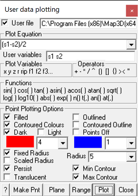
Plot Equation:
Defines the parameter that will be plotted, e.g. (f1-f2)/2 or equivalently (sig1-sig3)/2
The pull-down window allows you to store up to 20 different equations. These are stored between Map3D sessions in the map3d.ini file.
Plot Variables:
f1 f2 f3… data fields in the event file.
User defined variables (for example sig1 sig3 …) can be defined to indicate column headers corresponding to f1 f2 f3…
These can be defined in the comment line - any line leading with "*" or "#".
Simply provide the user defined plot variables as for example as follows:
* x y z sig1 sig2 ...
Functions:
sin() cos() tan() sine, cosine and tangent trigonometric functions
asin() acos() atan() Inverse trigonometric functions
sqrt() square root function
log() natural logarithmic function
log10() base 10 logarithmic function
abs() absolute value
exp() exponential function (antilogarithm)
n() t(,) normal and t-distribution
an() at(,) inverse normal and t-distribution
Location:
x y z coordinate of grid point.
Operators:
+ - * / ^ addition, subtraction, multiplication, division and exponentiation operators. Note that exponentials are computed first, followed by multiplication and division and finally addition and subtraction.
() [] {} styles of brackets. Pairs of brackets must match.
> maximum value. For example if the plot equation is specified as f1 > 10, the larger of f1 or 10 will be plotted.
< minimum value. For example if the plot equation is specified as f1 < 10, the smaller of f1 or 10 will be plotted.
Point Plotting Options:
Filled – points are filled with the specified colour, contoured colour and/or shaded.
Contoured Colours –fill colour is adjusted according to the magnitude determined from the Plot Equation.
Dark – fill colour is shaded to appear as light source shaded spheres using a dark rich colour scheme.
Light – fill colour is shaded to appear as light source shaded spheres using a bright shinny colour scheme.
Outlined – points are outlined with the specified colour or contoured colour.
Contoured Outline – points are drawn with contour colours adjusted according to the magnitude determined from the Plot Equation.
Contour Plane – enables or disables display of a contour plane (refer to Plane).
Fixed Radius – points will be plotted as spheres with a the specified Radius: parameter.
Scaled Radius – points will be plotted as spheres with radius scaled to the magnitude (determined from the Plot Equation) such that if the magnitude is less than the minimum of the contour range, the sphere is drawn with zero radius. If the magnitude equals the maximum of the contour range, the vector is drawn with the radius specified by the Radius: parameter.
Other:
Persist – when checked, the points will be re-plotted each time the model is reoriented, translated or zoomed. Since this may be time consuming for large models this option may not always be desired.
Translucent - draws the points as translucent spheres.
Zero Contour - when unchecked, contours below the minimum contour range are not drawn. This is useful for displaying contours where only the upper part of the contour range is important.
Make Point - adds of a new point.
Plane – enables setup of the contour plane.
Range – specify the minimum, maximum and interval for radius scaling and contouring.
![]() Plot regenerates the plot. This button can be placed on either the View Toolbar (Tools > View Toolbar Configure) or the Contour Toolbar (Tools > Contour Toolbar Configure).
Plot regenerates the plot. This button can be placed on either the View Toolbar (Tools > View Toolbar Configure) or the Contour Toolbar (Tools > Contour Toolbar Configure).