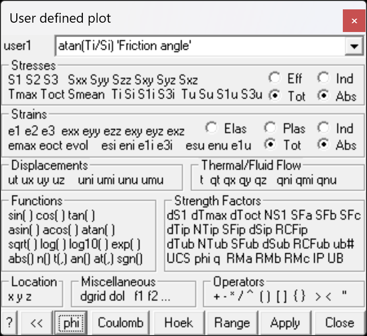
Contours a user defined stress component.
Stresses:
•S1 S2 S3 principal stress components σ1 σ2 σ3
•Sxx Syy Szz Sxy Syz Sxz Cartesian stress components σxx σyy σzz τxy τyz τzx
•Tmax maximum shear stress ½(σ1 - σ3)
•Toct octahedral shear stress τoct = ¹/3 [(σ1 - σ2)² + (σ2 - σ3)² +(σ3 - σ1)²]½
•Smean mean stress σmean = ¹/3 (σ1 + σ2 + σ3)
•Ti Si maximum shear and normal stress in the grid plane τip σip
•S1i S3i maximum and minimum stress tangential to the grid plane σ1i σ3i
•Tu Su maximum shear and normal stress in the ubiquitous-plane τub σub. The orientation of the ubiquitous shear plane is set using
•S1u S3u maximum and minimum stress tangential to the ubiquitous plane σ1u σ3u \]
•Effective/Total effective stress or total stress components. These options are only used in Map3D Thermal-Fluid Flow, as this code allows for calculation of steady state pore pressure distributions.
•Induced/Absolute induced stress or absolute stress components (i.e. the stress without the pre-mining stress contribution).
Strains:
•e1 e2 e3 major principal strain ε1 ε2 ε3
•exx eyy ezz exy eyz exz Cartesian strain components εxx εyy εzz εxy εyz εzx
•emax maximum shear strain ½(ε1 - ε3)
•eoct octahedral shear strain εoct = ¹/3 [(ε1 - ε2)² + (ε2 - ε3)² +(ε3 - ε1)²]½
•evol volumetric strain εvol = (ε1 + ε2 + ε3)
•esi eni maximum shear and normal strain in the grid plane εsi εni
•e1i e3i maximum and minimum strain tangential to the grid plane ε1i ε3i
•esu enu maximum shear and normal strain in the ubiquitous-plane εsu εnu
•e1u e3u maximum and minimum strain tangential to the ubiquitous plane ε1u ε3u
•Elastic/Plastic/Total elastic, plastic or total strain components. These options are only used in Map3D Non-Linear, as this code allows for calculation of non-linear strains.
•Induced/Absolute induced strain or absolute strain components (i.e. the stress without the pre-mining stress contribution).
Displacements:
•ut total displacement, its trend and plunge δt
•ux uy uz Cartesian displacement components δx δy δz
•uni displacement normal to the grid plane δni
•umi maximum displacement tangential to the grid plane δmi
•unu displacement normal to the ubiquitous plane δnu
•umu maximum displacement tangential to the ubiquitous plane δmu
Thermal/Fluid Flow:
•t temperature/head
•qt total flow, its trend and plunge.
•qx qy qz Cartesian flow components.
•qni displacement normal to the grid plane.
•qmi maximum displacement tangential to the grid plane.
•qnu displacement normal to the ubiquitous plane.
•qmu maximum displacement tangential to the ubiquitous plane.
Functions:
•sin() cos() tan() sine, cosine and tangent trigonometric functions.
•asin() acos() atan() Inverse trigonometric functions.
•sqrt() square root function.
•log() natural logarithmic function.
•log10() base 10 logarithmic function.
•exp() exponential function (antilogarithm).
•abs() absolute value.
•n() an() normal and inverse normal probability distribution. The argument used with the normal distribution is (Δσ1/s) which represents the excess major principal stress divided by the standard deviation (see ![]()
![]()
![]() ).
).
•t(,) at(,) t and inverse t probability distribution. The argument used with the t distribution is (Δσ1/(sg),n-2) where Δσ1 represents the excess major principal stress, s represents the standard deviation, n represents the number of data points, and g represents the factor [1 + 1/n + (σ3 - σm)²/s3²/(n-1)]½ where σm represents the mean value of σ3, and s3 represents the standard deviation of σ3.
•sgn() sign function return +1 for positive values, -1 for negative values and 0 for values with magnitude less than 10-12.
Strength:
•ds1 excess major principal stress Δσ1 = σ1 - ( UCS + q σ3 )
•dtmax excess maximum shear stress Δτmax = ½(σ1 - σ3) - [ UCS + ½(σ1+σ3) (q-1) ]/(q+1) = [σ1 - ( UCS + q σ3) ]/(q+1)
•dtoct excess octahedral shear stress Δτoct = τoct - [ UCS + (q–1) σmean ] √(2) /(q+2)
•NS1 probability using the Normal distribution N(Δσ1 /std)
•SFA Strength/Stress can be determined for Mohr-Coulomb as ( UCS + q σ3 )/ σ1
| or for Hoek-Brown as [ σ3 + √(m σcσ3 + s σc²) ] / σ1 |
•SFB Strength/Stress can be determined for Mohr-Coulomb as ( UCS + q σ3 - σ3 )/(σ1 - σ3)
| or for Hoek-Brown as [ σ3 + √(m σcσ3 + s σc²) ] / (σ1 - σ3) |
•SFC Strength/Stress can be determined for Mohr-Coulomb as [ UCS + ½(σ1+σ3) (q-1) ]/[ ½(σ1 - σ3)(q+1) ]
| or for Hoek-Brown as {√[ 1/16 m²σc² + ½(σ1 + σ3) mσc + s σc²] - ¼ mσc}/(σ1 - σ3) |
•dTip excess in-plane shear stress Δτip = τip - [ Cohesion + σip tan(φ) ]
•NTip probability using the Normal distribution N(Δτip /std)
•SFip Strength/Stress can be determined as [ Cohesion + σip tan(φ) ] / τip
•dSip excess in-plane wall stress Δσip = [ 3 σ1i - σ3i ] - UCS
•RCFip Rock Condition Factor for the in-plane wall stress RCFip = [ 3 σ1i - σ3i ]/UCS
•dTub excess ubiquitous-plane shear stress Δτub
•NTub probability using the Normal distribution N(Δτub /std)
•SFub Strength/Stress can be determined as [ Cohesion + σub tan(φ) ] / τub
•dSub excess ub-plane wall stress Δσub = [ 3 σ1ub - σ3ub ] - UCS
•RCFub Rock Condition Factor for the ub-plane wall stress RCFip = [ 3 σ1ub - σ3ub ]/UCS
•UB# Plots the UB set number (1, 2 or 3) that has the largest value of Δτub
•UCS phi q Mohr-Coulomb strength parameters defined using ![]() Plot > Strength Factors > Rockmass Strength Parameters note that these parameters are only defined if you have specified the Mohr-Coulomb or Druker-Prager strength criterion
Plot > Strength Factors > Rockmass Strength Parameters note that these parameters are only defined if you have specified the Mohr-Coulomb or Druker-Prager strength criterion
•RMa Rock mass strength defined for Mohr-Coulomb as ( UCS + q σ3 )
| or for Hoek-Brown as [ σ3 + √(m σcσ3 + s σc²) ] |
•RMb Rock mass strength defined for Mohr-Coulomb as ( UCS + q σ3 - σ3 )
| or for Hoek-Brown as [ √(m σcσ3 + s σc²) ] |
•RMc Rock mass strength defined for Mohr-Coulomb as [ UCS + ½(σ1+σ3) (q-1) ]/(q+1)
| or for Hoek-Brown as {√[ 1/16 m²σc² + ½(σ1 + σ3) mσc + s σc²] - ¼ mσc}/2 |
•IP In-Plane strength defined using Mohr-Coulomb as [ Cohesion + σip tan(φ) ]
•UB Ubiquitous strength defined using Mohr-Coulomb as [ Cohesion + σub tan(φ) ]
•sc Hoek-Brown strength parameter defined using ![]() Plot > Strength Factors > Rockmass Strength Parameters note that this parameter is only defined if you have specified the Hoek-Brown strength criterion
Plot > Strength Factors > Rockmass Strength Parameters note that this parameter is only defined if you have specified the Hoek-Brown strength criterion
Location:
•x y z coordinate of grid point.
Miscellaneous:
•Dgrid distance to the nearest surface from each grid point.
•Dol distance to the nearest grid Dgrid divided by the grid spacing Lgrid.
•f1 f2... user defined material parameters. These can be defined using Plot > Properties > Material Properties > User defined Parameters.
Operators:
•+ - * / ^ addition, subtraction, multiplication, division and exponentiation operators. Note that exponentials are computed first, followed by multiplication and division and finally addition and subtraction.
•() [] {} styles of brackets. Pairs of brackets must match.
•> maximum value. For example if the plot equation is specified as s1 > 10, the larger of s1 or 10 will be plotted.
•< minimum value. For example if the plot equation is specified as s1 < 10, the smaller of s1 or 10 will be plotted.
• " " comment.
Other:
•phi: atan(Ti/Si) plots the friction angle necessary to resist slip on a fault, joint set or bedding plane oriented in the same way as the grid plane.
•Mohr-Coulomb: 60 + S3*tan(45+30/2)^2 plots the strength for a Mohr-Coulomb criterion with a UCS of 60 and friction angle of 30°. The equation UCS + S3*q or alternatively UCS +S3*tan(45+phi/2)^2 could also be used here if the strength parameters have been previously defined using ![]() Plot > Strength Factors > Rockmass Strength Parameters.
Plot > Strength Factors > Rockmass Strength Parameters.
•Hoek: S3 + sqrt( 0.1*60*S3 + 0.005*60^2 ) plots the strength for a Hoek-Brown criterion with a sc of 60 and m of 0.1 and s of 0.005.
•Range – sets the contour range.
•Plot – regenerates the contour plot.
The pull-down window allows you to store up to 20 different equations. These are stored between Map3D sessions in the map3d.ini file.